Mathematical Visualization
Mathematical concepts can produce some really cool visualizations. However, a lot of times these concepts are very abstract and complex on a theoretical level, whereas implementing them in code is not. For that reason, I struggled to implement some of these. In the end, I was able to put my implementation together by looking at various blogs and websites, comparing people’s implementations in order to understand the concept at hand. For that reason, I am accompanying each project with a short description, in layman’s terms, of the concept and the implementation method. From my understanding, nobody is going to bother downloading my code and running it. But someone might, at the very least, stumble upon this website with these pretty images of what they want to do and it might help them understand how to do it without having to bother downloading git repos and looking at code of a platform they’re not familiar with.
Index
- 2D Fractals see on github
- Raymarched Fractals see on github
- Buddhabrot see on github
- Knots see on github
- Lorenz System see on github
- Mobius Strip see on github
- Cellular Automata see on github
2D Fractals see on github
Implementation of the following fractal formulas:
- Mandelbrot
- Multibrot
- Julia
- Multijulia
- Burning Ship
- Tricorn
- Barnsley Fractal
- Magnet Fractal
- Newton Fractal w/ Transformation Vector
- Burning Julia
- Conjulia
And the following rendering techniques:
- Escape-Time
- Smooth
- Lyapunov Exponent
- Orbit Trap
- Pickover Stalk
- Edge Detection
- Normal Mapped
- Hue
- Cheap Interior Distance Estimation
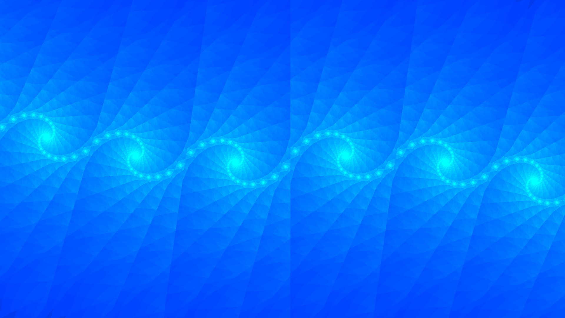
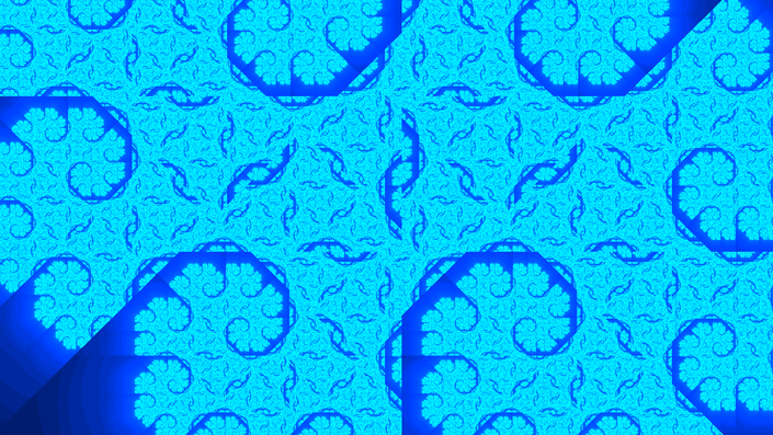
These fractals are the representation of a set of complex numbers Z(x+yi) on the complex plane. There isn’t a deterministic way to find out if a point is in one of these sets. Instead, we iterate through every point in the plane and check if it belongs. Imagine your image represents the complex plane; every pixel represents a complex number Z(x + iy). The Mandelbrot set is given by applying the equation Z^2+c, where c is the first value of Z, over and over again. If this function escapes to infinity (goes really high), the point does not belong in the Mandelbrot set. This is called an escape-time fractal because of this. A way to check if a point escapes is to see if cabs(Z) > 4, because in general, if it goes over 4, it will increase exponentially towards infinity. If your point does not escape after X iterations, you can assume if belongs in the set. You can then color that pixel, for example, in function of the number of iterations it took for the point to escape.
Different fractals will have different equations, it is generally just a matter of swapping that part in your code. Do remember that these are complex numbers, meaning that they are 2 dimentional and have their own operations.

Raymarched Fractals see on github
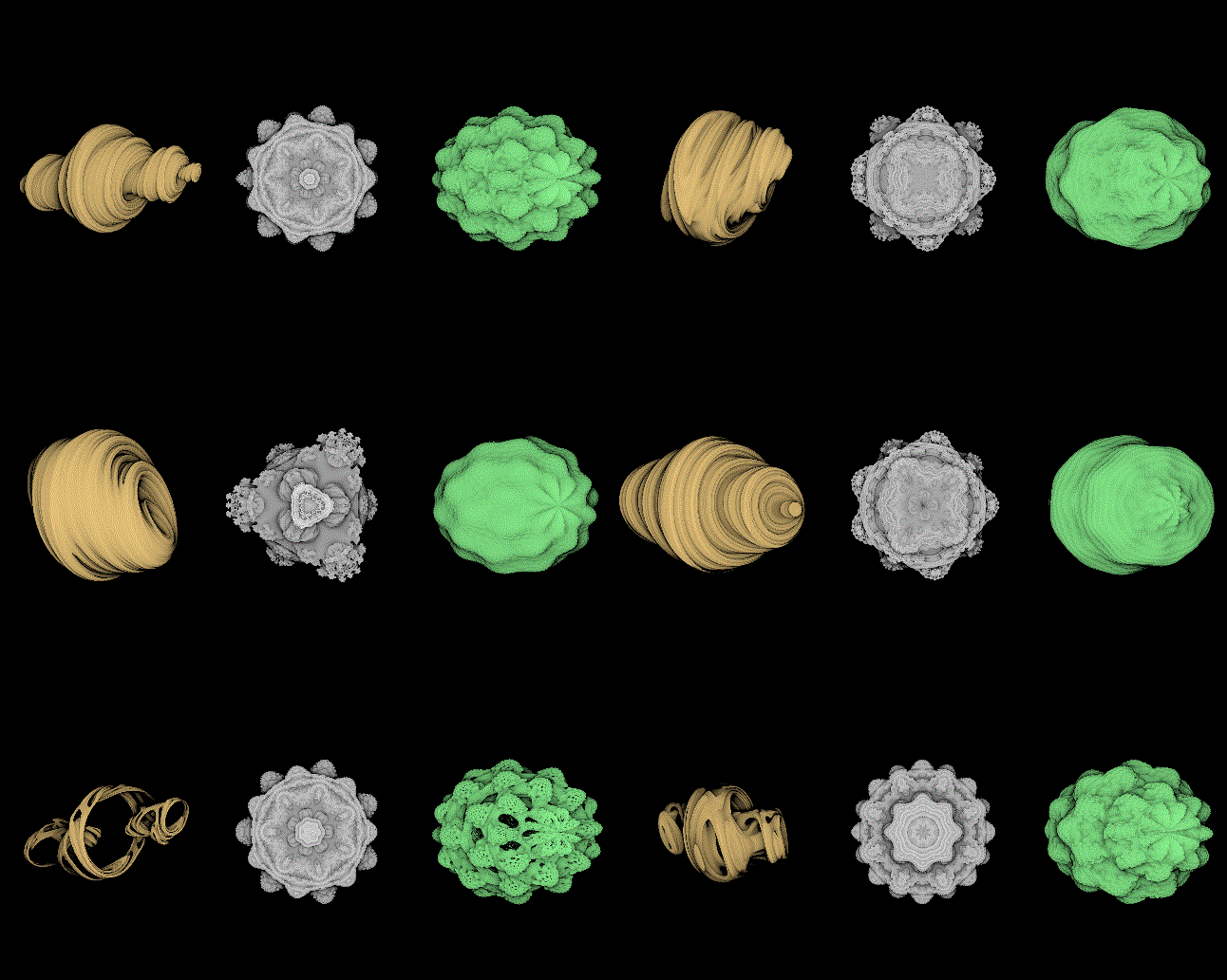
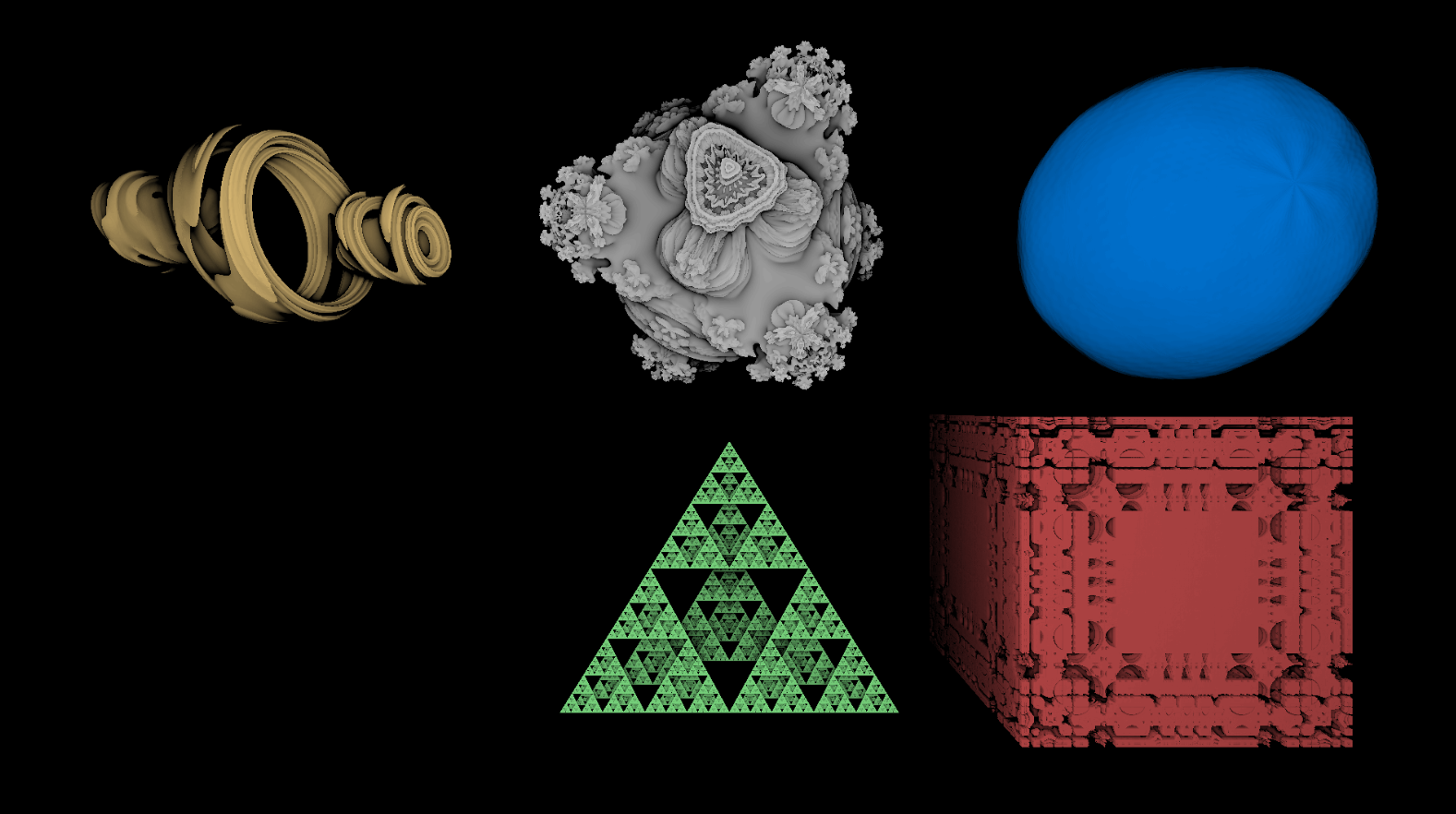
First experimentation with Raymarching. Implemented in Unity as a Post-Processing effect. The Signed Distance Functions were taken from Shadertoy, and for the rendering it is a mixture of fake iteration-based Ambient Occlusion and Phong shading.
These fractals, on the math level, are somewhat like black magic to me. Instead of trying to explain how they exist, I will go over the implementation details. The basic part is this: there is a magic function, called SDF (Signed Distance Function), which gives you the distance between any point and the closest point in an object. These functions are somewhat easy to understand for primitives like spheres and cubes, but some intelligent people have created SDFs for the fractals you see displayed. But how do you render with an SDF? Using raymarching. For every pixel in your image, shoot a ray out of your camera and calculate the distance to the nearest point in the surface using an SDF of your choice. Move the ray forward by that amount. Repeat this until you intersect with the object (meaning that the distance will be <.001 ). You move the ray forward by the distance of the closest point because it ensures that you can never go inside of the object. If the ray was pointed straight at the object, it would simply land at the nearest point and the next distance evaluation would be 0. This is rather hard to convey in text, so please take a look at the images in this blog: Reference.
You can find many SDFs in a website called Shadertoy. They are usually in the code under a function called map(), which is used to sample multiple SDFs simoultaneously.
Buddhabrot see on github
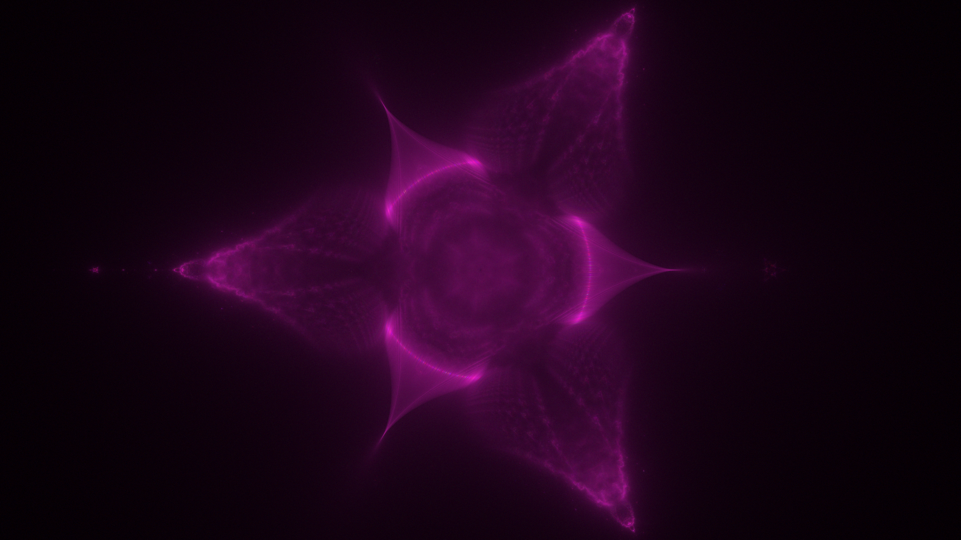
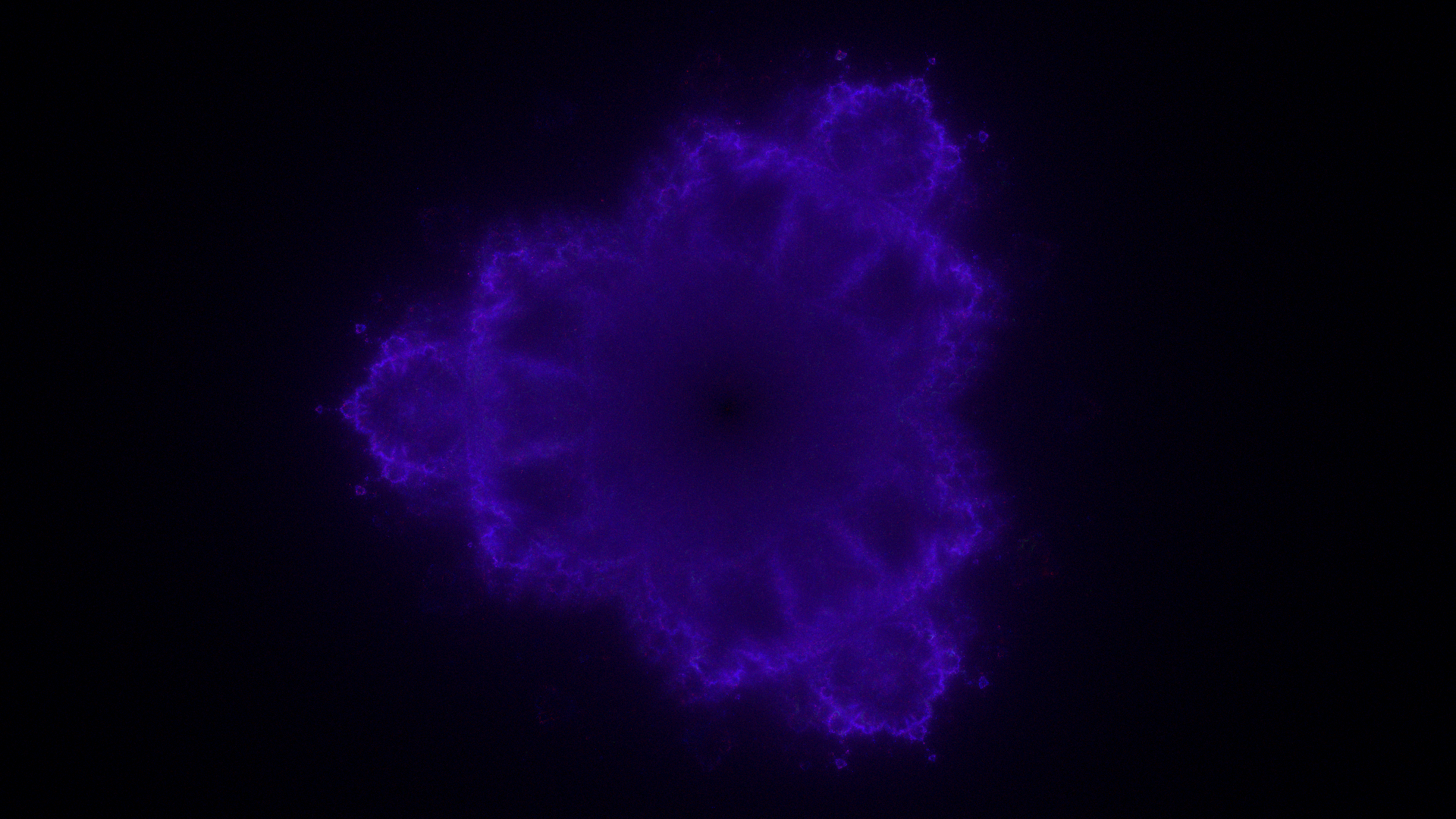
Mandelbrot set variants rendered with a histogram.
A Buddhabrot is created using the same algorithm we used to determine if a point belongs in the Mandelbrot set, but with a twist. Our image serves as a representation of the complex plane. When we initialize Z(x + iy), we are converting our pixel into a complex number. Whenever we iterate Z^2+c, Z will change, meaning it will be located in a different place of the Complex Plane. A different pixel in our image. A Buddhabrot is rendered by keeping track of how many times a pixel was visited by other pixels which escaped (and do not belong in the Mandelbrot Set). This can be achieved by having a grid of integers for every pixel which get incremented whenever they are visited. In the end, it can be rendered as grayscale by making the values linear. For colored rendering, you compute this grid 3 times, one for each color channel (RGB), except every time you do you change the maximum number of iterations. This rendering method can also be applied to other escape-time fractals.
Knots see on github
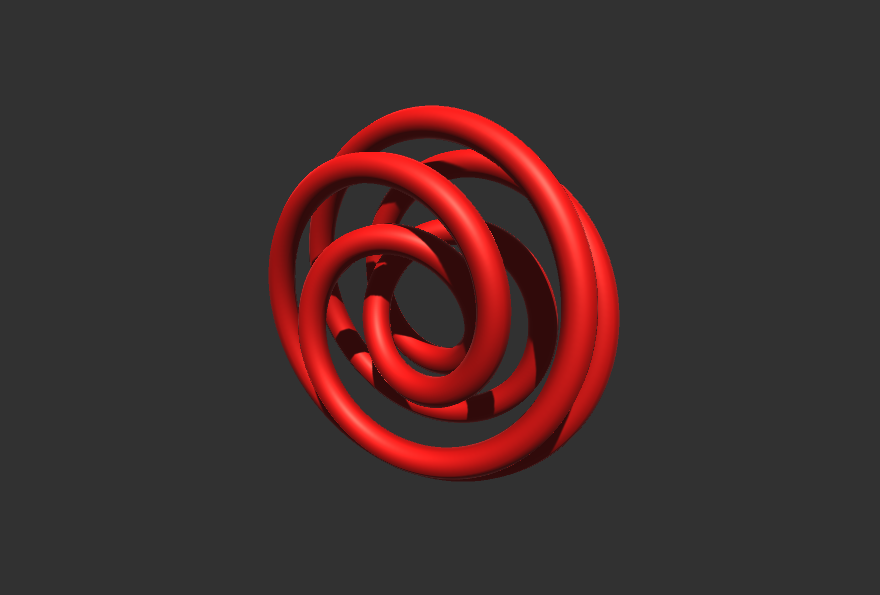
Generation and triangulation of mathematical knots.
Simply put, knot is a closed curve that cannot be untangled. I don’t quite understand the theory behind them, but I will explain how I implemented them.
Given a variable u, which ranges from ]0 ; 2π[, there are a set of functions that transform u into a 3D point belonging to the knot. F(0) = F(2π), since a knot is a closed loop. The actual range for u and the functions used depend on the knot you are trying to generate. I sourced mine from Paul Bourke’s website Having the points in the knot, it is now necessary to triangulate them. To do this, calculate the normal vector N of the edge between every point and the next. Afterwards, for every point, generate n vertices evenly spaced in a circumference of radius N (see github for visualization). In the end, it is just a matter of combining the vertices at each point and triangulating them.

Lorenz System see on github
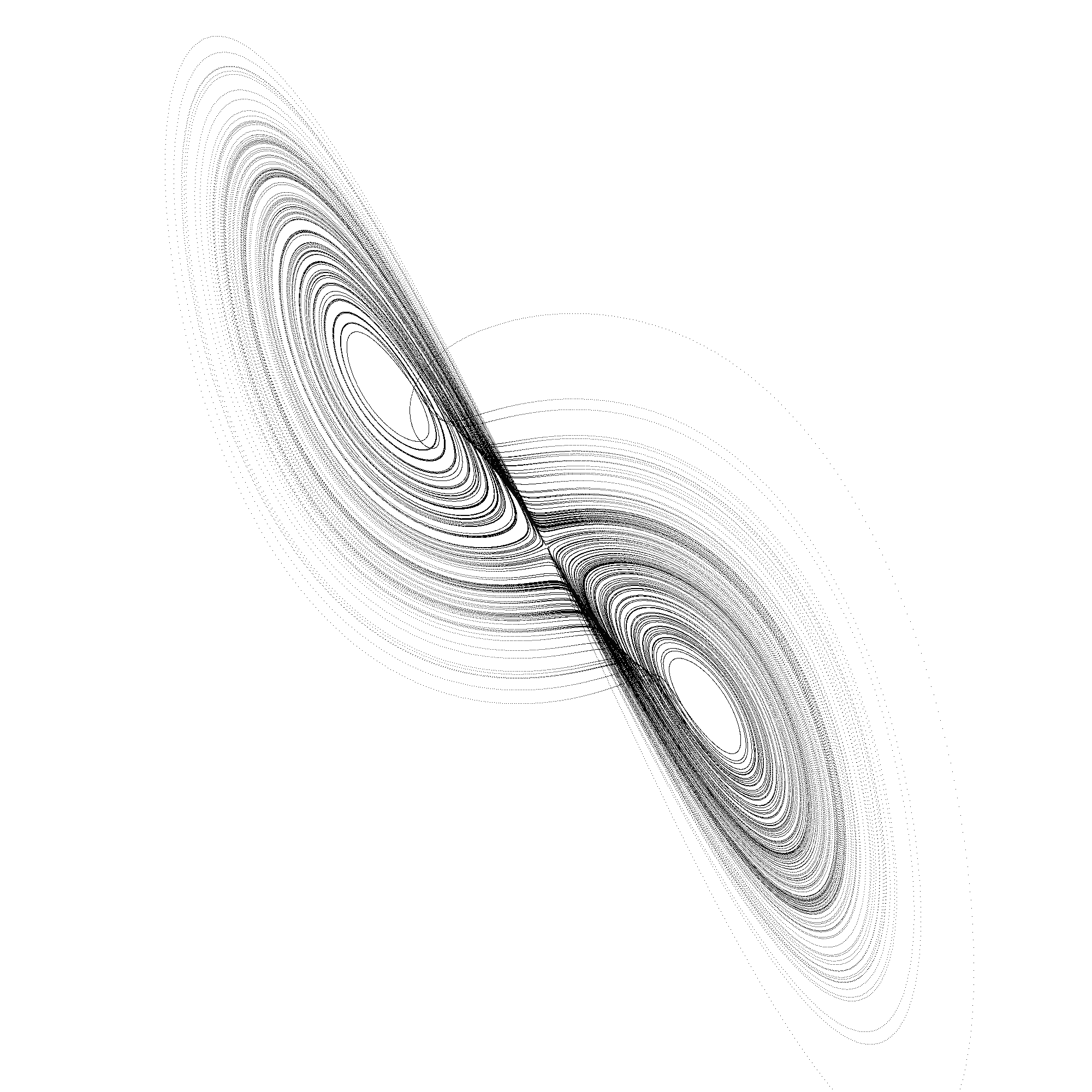
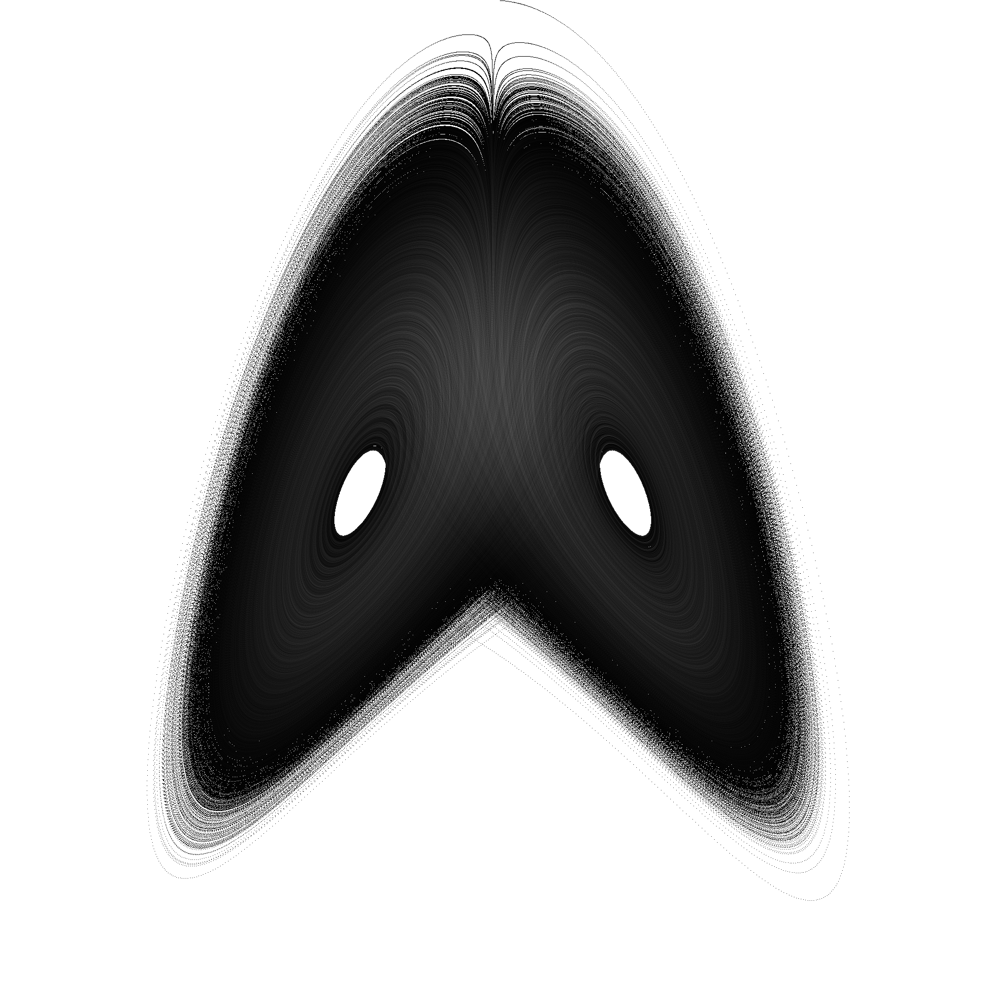
Visualization of a Chaotic 3 variable system with a histogram.
The lorenz system is a set of 3 differential equations. These equations tell you how much the position of a point varies. There are 3 equations, one for each axis (XYZ). These equations rely on the input of 3 predeteremined variables named ρ, σ and β. These variables are set at the start of the simulation and don’t change. Possible values for them are, for example, ρ = 28, σ = 10, and β = 8/3.
To render a lorenz system, you start with a non-zero point P. Solve the differential equations for the point. Add the output to the current point’s position. Render the point. Repeat. In order to obtain smooth results, multiply the result of the equations by something like 0.01. This ensures that the point moves very little each time, which generates more data.
Mobius Strip see on github
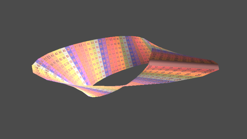
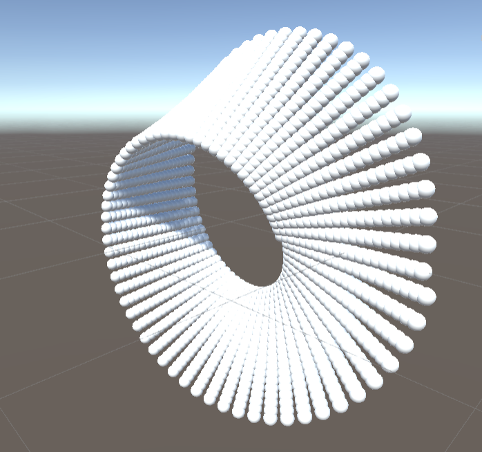
2 Variable parametric surface plotting and triangulation.
A Mobius Strip is a one-sided surface. If you were to somehow be walking on one, you would be find yourself on the other side of where you started without having crossed an edge. It can be implemented as a parametric surface: Imagine you have a plane (u, v), going from u [0; 2π[ and v [-1; 1]. Given a point in this plane, the parametric surface equations will tell you where it will end up in three dimensions. so from P(u,v) you get P(x,y,z). It is essentially a deformation of the plane. In order to render it, generate a grid that will correspond to your plane. Triangulate it, as a normal grid. Then calculate the transformed position for every vertex. The vertices will change place but the triangles will remain the same.
Cellular Automata see on github
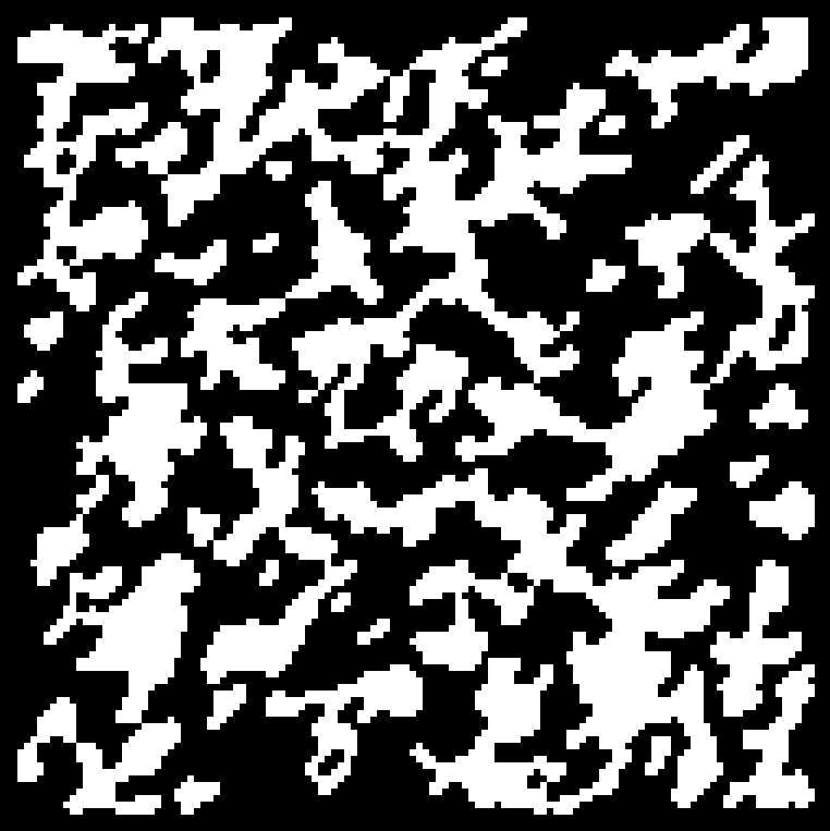
Simulation of individual cell behaviour being based on neighbour status.
Cellular Automata operates on a grid, where a cell can be either on or off. Every time the grid is refreshed, every cell will look for the status of its neighbours in order to set its own status. The rules used can vary; the one I implemented stated that every cell will adopt the status of the majority of its neighbours. So if most are a 0, it will turn to a 0 as well. This method is often used in procedural generation, mainly in cave generation. A well known application of this technique is Conway’s Game of Life.
